As an example let’s take a group of five friends who we will represent by the first initial of their names as a set: \(\{\mathrm{\,S, C, A, L, M\,}\}\). The elements of this set of people, like the elements of any set, can be arranged in different orders. For example, the order of the elements as we just happened to write them \((\mathrm{S\; C\; A\; L\; M})\) is one arrangement, and we can also shuffle them around to get a different arrangement like \((\mathrm{C\; A\; M\; L\; S})\).

Each ordered arrangement is called a permutation of the set. How many permutations can be made from a set with \(n\) elements? It is straight-forward to count. We can choose any element of the set to be in the first position of the permutation, so there are \(n\) choices, which leaves \(n-1\) choices for the second position, \(n-2\) choices for the third position, and so on until for the \(n\text{th}\) (and therefore last) position of the permutation there is only one element of the set remaining to choose from.

Multiplying the number of choices for each position of the permutation gives the total number of possible permutations: \(n(n-1)(n-2)\dots(1).\) In other words, the product of all positive integers less than or equal to \(n\). That product is known as the factorial of \(n\) and is written \(n!\):

So there are \(5! = 5 \cdot 4 \cdot 3 \cdot 2 \cdot 1 = 120\) ways to permute a set of five friends. Writing any two of those permutations in two-line notation with one above the other allows us to read off a secret santa assignment for the group:

If we read the top line of as the list of gift givers and the bottom line as the gift recipients, then each santa is assigned to give a gift to the person in the bottom line directly beneath them. So \(\mathrm{S}\) gives a gift to \(\mathrm{C}\) who gives a gift to \(\mathrm{A}\) and so forth.

A permutation of santas (or anything else) can be represented as a directed graph, as in Figure 1, or more compactly by listing its cycles: \((\mathrm{S\; C\; A\; M})(\mathrm{L})\). To see that the cycle notation is equivalent to the graph, read each cycle from left to right and insert the implied arrow from the last element back to the first: \((\mathrm{S \to C \to A \to M \to S})(\mathrm{L \to L})\). Note that any 1-cycles can be implied and are usually left out when writing a permutation in cycle notation, so an equivalent way to write our example permutation is simply as \((\mathrm{S\; C\; A\; M})\).

But note also that a permutation containing any 1-cycles defines an invalid secret santa assignment! The example permutation above has \(\mathrm{L}\) giving a gift to herself, which is against the rules.

A permutation with no 1-cycles — in other words, a permutation in which no element is left in its original position so that the entire set has been de-arranged — is called a derangement. One way to derange our example group of secret santas is

Or equivalently, decomposed into its cycles, \((\mathrm{S\; C\; A})(\mathrm{M\; L})\).

So the problem of generating a valid secret santa assignment is equivalent to generating a derangement. Some algorithms for uniformly generating random derangements are presented in the next section. But first we need a way to calculate \(D_n\), the number of derangements that can be made from a set with \(n\) elements.

Counting derangements is a trickier than counting unrestricted permutations. We proceed by counting the permutations with at least one 1-cycle, the non-derangements. First we’ll define the subsets \(H_p\) to contain all of the permutations on \(n\) with the \(p^{\text{th}}\) element fixed in its original position (an element that stays in its original position in a permutation is called a “fixed point”). This gives \(n\) such subsets \(\mathrm{(}H_1 \ldots H_n\mathrm{)}\) each containing \((n-1)!\) permutations (because with one element fixed, there are \((n-1)!\) ways to permute the remaining elements).

We know that the subsets \(H_p\) contain only non-derangements since every member has a fixed point. And since together the \(H_p\) contain every non-derangement with the \(p^{\text{th}}\) element fixed, we know that they contain all possible non-derangements. That means to find \(D_n\) we just need to subtract the size of the union of all the \(H_p\) subsets from the total number of permutations (which we know is \(n!\)):

But finding the size of \(\cup H_p\) is not straightforward. If we simply multiply the number of subsets by their size \(n\cdot(n-1)!\) we over count because the subsets \(H_p\) are not disjoint: some non-derangements belong to more than one subset. Specifically, every pair of subsets of \(H_p\) share \((n-2)!\) permutations with at least two fixed points; every 3-tuple of subsets share \((n-3)!\) permutations with at least three fixed points; and so on.

To visualize this, it helps to draw out each \(H_p\) for a small set. The table below shows each \(H_p\) subset for the set \(\{\,a, b, c, d\,\}\):

Notice that the first column, \(H_1\), has "a" fixed in the first position; the second column has "b" fixed in the second position; etc. Note also that the \(H_1\) and \(H_2\) columns share every permutation with the first and second position fixed ("abcd" and "abdc").

To weed out the duplicates, we need to subtract the number of permutations with at least two fixed points multiplied by the number of pairs of \(H_p\) subsets. But that will leave us with an under count because it will result in some permutations with three or more fixed points being excluded, so we must add those back in. We need to continue this inclusion-exclusion process until we’ve considered the number of permutations which fix all \(n\) elements in \(H_p\) taken \(n\) at a time:

where \(\binom{n}{k}\) gives the binomial coefficients which you may remember from math class can be interpreted as the number of ways to choose \(k\) objects from a set of \(n\) objects when order doesn’t matter. It can be written in terms of factorials:

Now we can calculate the number of possible non-deranged permutations. To get \(D_n\), we just subtract it from the total number of possible permutations. When we substitute the expression for \(\lvert \bigcup H_p \rvert\) into equation \eqref{eq:up} then expand the binomial coefficients and factorials, this becomes:

And we’ve answered our first question: Given a group of size \(n\), there are \(D_n =n!\sum_{k=0}^n(-1)^k\frac{1}{k!}\) ways to make a valid secret santa assignment. To calculate the number of valid assignments between our five example friends, then, we have

The first nine values of \(D_n\) are listed in the table below.

This is OEIS sequence A000166. The number \(D_n\) is known as the subfactorial of \(n\) (usually written \(!n\)). It is also a special case of the rencontres numbers which enumerate partial derangements (derangements with specified numbers of 1-cycles).

Notice that the summation in equation \(\eqref{eq:dn}\) is the \(n^{\text{th}}\) partial Maclaurin expansion of \(e^{-1}\), so that

Because the series converges rather quickly, \(\frac{n!}{e}\) is a good approximation even for even small values of \(n\).

The probability that a permutation is a derangement is \(D_n\) divided by the number of all possible permutations \(n!\). This answers the second question asked in the introduction: The probability that at least one secret santa participant will draw their own name is \(1 - \frac{D_n}{n!} \approx 1 - \frac{1}{e} \approx 63\%\). That may seem high, but the mean of the geometric distribution is \(e\) so you can expect to draw a valid derangement after 2 or 3 attempts (restarting each time someone draws their own name). There is a nearly 99% chance of having drawn a derangement after 10 attempts \((1 - (1 - \frac{1}{e})^{10} \approx 98.9\%)\).

Beyond counting mere derangements there are more elaborate constraints and questions we could consider, the sorts of things investigated by statistics of random permutations and generating functions. We haven’t even answered the third question from the introduction yet (“What is the probability that two people will draw each other’s names?”). I hope to return to this article in the future when I have more time and a better grasp of combinatoric tools to look into some of those questions.

If my explanation above of how to derive \(D_n\) was not clear, don’t worry. Counting derangements is frequently used as an example application of the inclusion-exclusion principle, so better explanations can be found on the web and in almost any introductory combinatorics textbook. See, for example, Professor Howard Haber’s handout on the inclusion-exclusion principle [PDF]. There are also several other methods for deriving and proving the formula for \(D_n\), including those that first derive the recurrence relation \(D_n = (n-1)(D_{n-1} + D_{n-2})\) and then solve it by iteration or by the method of generating functions. For a solution via generating functions see Jean Pierre Mutanguha’s “The Power of Generating Functions”.

There are a few utility functions that we might want while exploring and debugging our algorithms. First of all, the ability to calculate \(D_n\), the number of derangements in a set of size \(n\). Here is a straightforward translation of \(\eqref{eq:dn}\) to Python:

Next up is a way to generate all \(n!\) permutations of a set. Several algorithms for generating permutations are well-known. Most classic is an algorithm which produces permutations in lexicographical order described by Knuth in 7.2.1.2 Algorithm L. Other techniques produce all permutations by only swapping one pair of elements at a time (see the Steinhaus-Johnson-Trotter algorithm which Knuth gives as Algorithm P).

But in our case the Python standard library provides a function for generating permutations (in lexicographical order) so we’ll just use that:

Another helpful function would be a way to decompose permutations into their cycles to make them easier to visualize (taking \((0, 1, 2,\cdots, n-1)\) to be the identity permutation). To find the cycles in a permutation, start with the first element and then visit the element it points to (the element in its position in the identity permutation), and then visit the element that one points to and so on until we get back to the first element. That completes a cycle containing each of the elements visited, add it to a list. Now start over with the first unvisited element. Repeat until there are no more unvisited elements.

Below is an implementation of that algorithm. It requires storage for the list of cycles (the cycles variable), a way to keep track of unvisited elements (the unvisited variable, which starts as a copy of the input but has elements removed as they are visited), and a way to keep track of the first element in a cycle so that we know when we’ve returned to it (the variable called first below):

As an example, let’s see the cycles in \(\{1, 2, 4, 3, 0\}\mathrm{:}\)

Notice this agrees with the same cycles we found way back in our first example of a permutation (where \(\mathrm{S}=0, \mathrm{C}=1, \mathrm{A}=2, \mathrm{L}=3, \mathrm{M}=4\)) \(\eqref{eq:perm}\).

Finally, it will be handy to have a function that can test whether a permutation is a derangement or not. One way to do that would be to call decompose() on the permutation and then check if there are any 1-cycles in the decomposition. The nice thing about that method is that it generalizes so we could use it to check if the permutation contains any cycles \(\leq m\) for any \(m\).

But if we only care about derangements (the case where \(m=1\)), it is simpler (and faster) to just iterate over the elements of the permutation and check if they are in their original position. If any are, we can immediately return False, the permutation is not a derangement.

The first time I sat down to write a secret santa algorithm, my instinct was to try a backtracking approach and ended up with something like the code below. The idea behind the backtracker is to iteratively build a derangement by randomly selecting an element from the identity arrangement, and then checking if the resulting partial permutation is a derangement. If it is not a derangement, undo (backtrack) the last choice and try again. If it is a derangement, randomly choose one of the remaining elements and check again. Repeat until you’ve deranged all \(n\) elements:

As written, backtracker() is fast and will produce any possible derangement (and in only ~20 lines of Python), so it could be used for secret santa. However, as the decades fly by your friends might begin to suspect that the same assignments seem to be ‘randomly’ generated fairly often. They would be right: backtracker() does not produce derangements with uniform probability. Even though each element in the derangement is chosen from the remaining elements of the input set with uniform probability, the number of possible derangements is dependant on which numbers happen to have been chosen first.

For example, let’s look at the probability that backtracker() will produce \((5, 0, 1, 2, 3, 4).\) The first number can be anything but 0, so there are \(6-1=5\) ways to choose that. The second number can be any of the remaining 5 numbers except 1, so there are 4 ways to choose that. The third number can be any of the remaining 4 numbers except 2 which leaves 3 possibilities. The fourth element can be any of the remaining numbers except for 2 which leaves 2 possibilities. The fifth element can not be 4, so there is only one way to derange the last two elements. If we take the product of those probabilities we get \(\frac{1}{5} \cdot \frac{1}{4} \cdot \frac{1}{3} \cdot \frac{1}{2} = \frac{1}{120}.\)

If you do a similar calculation for the probability that backtracker() would produce \((2, 3, 5, 4, 0, 1)\) you should get \(\frac{1}{360}.\) Not only are the probabilities for generating those two derangements significantly different from each other but they also both differ from the expected probability of \(\frac{1}{265}\) if every one of the \(D_6\) derangements had an equal probability of being generated. 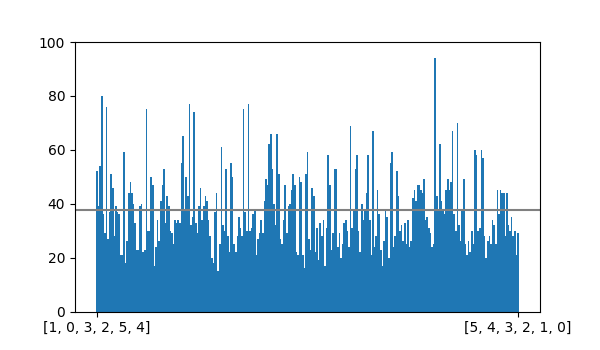I generated 10,000 derangements of length 6 with backtracker(), and sure enough \((5, 0, 1, 2, 3, 4)\) was generated 94 times while \((2, 3, 5, 4, 0, 1)\) was generated only 20 times. The graph below shows a plot of counts for every 6-derangement over the 10,000 runs:

Instead of building derangements by randomly selecting elements and checking if the result is a derangement, we could simply generate all possible permutations, filter out the non-derangements, and then randomly select one of the derangements to return. The nice thing about that approach is that we could enforce any other constraints we want in the filter step (maybe we want a minimum cycle length or have a “blacklist” of people who should not be assigned to each other) and we can still be confident we would select a valid secret santa assignment with uniform probability (since we have generated all of them it is easy to select one at random).

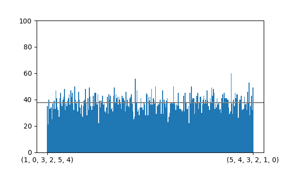
Below you can see a bar graph of the counts after producing 10,000 derangements of length 6 with generate_all(). It looks much more uniform than backtracker() at least. One tool we can use to gauge how closely our counts match what we should expect from a uniform distribution is the chi-squared statistic:

where \(O_i\) are our observed counts and \(E_i\) are the expected counts for each derangement (which in our case is \(1/D_6\cdot 10000 \approx 37.7\)). For my data I calculated \(\chi^2 \approx 261.75\). If we check that against the chi-squared cumulative distribution function with k-1 degrees of freedom (where k is the number of data points, 265 in this case), we get a p-value of about 0.53. The p-value is the probability that our \(\chi^2\) value would be least 261.75 if our counts were uniformly distributed. Usually if p<0.05 it would be prudent to question whether the data fits a uniform distribution. On the other hand if p>0.99 or so we could be confident it is uniform, but we might question whether it is random. A p-value of 0.53 should leave us confident that generate_all() randomly generates derangements with uniform or very nearly uniform probability.

But there are two major problems with generate_all(): it is slow (because we have to generate all \(n!\) permutations), and it uses a lot of memory (because we have to store all \(D_n\) derangements). \(D_{12} = 176,214,841\), for example, so even if we implemented our permutations in some memory efficient way (say an array of one byte per element), we would need over 1GB of memory just to store all of the derangements before returning one. Running generate_all() with \(n>11\) runs my desktop out of RAM after about a minute and crashes the Python interpreter. And in the grand scheme of things 12 is not such a huge number.

We can do better than the backtracker and generate_all algorithms above by combining the best aspects of each: generate a single random permutation and check if it is a derangement. If it is, return it; otherwise, try again by generating another random permutation. That should be much more efficient than generating and storing all possible derangements, and as long as we can generate permutations with uniform probability we will also generate derangements with uniform probability.

A well-known algorithm for creating a random permutation by shuffling a given arrangement is to simply select one of the elements at random, set that as the leftmost element of the permutation, and then repeat by selecting one of the remaining elements at random until all of the elements have been selected. This is known as the Fisher-Yates shuffle named for two statisticians who described a paper-and-pen method for shuffling a sequence in 1938. The computer version of the algorithm — popularized in Chapter 3 of Knuth’s The Art of Computer Programming (“Algorithm P (Shuffling)”) — usually shuffles an array in place. It does this by iterating through the array from left to right swapping the element at the index with a random element to the right of the index. Once an element has been swapped left it is in its position in the generated permutation. Repeat to the end. For a good visualization of Fisher-Yates (and how it compares to less efficient algorithms) see Mike Bostock’s Fisher-Yates Shuffle.

The shuffle_rejection() algorithm below repeatedly shuffles a list using Fisher-Yates until the resulting permutation is a derangement:

Notice that in the Fisher-Yates algorithm the range of the random index k includes the index of the current element i. In other words, elements can swap with themselves creating a 1-cycle. That is necessary, of course, to generate all possible permutations. If the algorithm is changed so that k ranges only from \(i < k < n\) so that it does not include i, then the algorithm will produce only permutations with a single n-cycle. This is known as Sattolo’s algorithm, and it generates n-cycles with uniform probability.

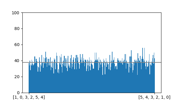
The bar graph above summarizes the results of generating 10,000 derangements of size 6 with shuffle_rejection(). It appears to be uniform as expected. It is also fast and simple, which makes it perfectly suitable for generating secret santa assignments (and is, in fact, what I use in sinterbot, my secret santa tool).

One inelegance of shuffle_rejection() is that it generates any number of random permutations just to throw them away. It is possible that it would never actually generate a derangement and just keep generating and rejecting permutations all day. In reality derangements are common enough that that is not a practical concern (it finds close to 20,000 derangements of length 6 per second on my old desktop). But is there a way to directly generate derangements with uniform probability without needing to backtrack or reject non-deranged permutations?

Yes. In 2008 Martínez et al. published one such algorithm (“Generating Random Derangements,” 234-240). It is similar to Sattolo’s algorithm, but instead of joining every element into a single n-cycle, it will randomly close cycles at a specific probability which ensures a uniform generation of derangements. Here is a nice set of slides that goes through their algorithm step by step.

Jörg Arndt provides an easier to follow (in my opinion) version of the algorithm in his 2010 thesis Generating Random Permutations. (It’s a short book that includes several useful algorithms.) This Python implementation more closely follows his version:

Arndt’s implementation is in C with a precomputed lookup table for the ratio calculated on the prob = r * Dn(r-1)/Dn(r+1) line. Even then he reports it is only slightly faster than the rejection method. This Python implementation is actually about twice as slow as the rejection method in my tests.

But one advantage of generating derangements directly as in rand_derangement() is that it can be generalized to generate derangements with minimum cycle lengths. Arndt shows how that can be done in his thesis.

There are other ways to generate random derangements that I’ve not covered in this post. Earlier this year J. Ricardo G. Mendonça published two new algorithms for [almost-]uniformly generating random derangements: “Efficient generation of random derangements with the expected distribution of cycle lengths,” Computational and Applied Mathematics 39, no. 3 (2020): 1-15.

First create a config file with a list of participants' names and email addresses. The config file may also specify constraints for minimum cycle length and a blacklist. See sample.conf for a full example:

The format is Name: emailaddress. Only the email addresses need to be unique.

Then run sinterbot derange to compute a valid assignment and save it to the config file:

sinterbot will not allow you to re-derange a config file without passing the --force flag.

Now if you want you can view the secret santa assignments with sinterbot view xmas2020.conf. However, if you’re a participant that would ruin the suprise for you! Instead you can email each person their assignment without ever seeing them yourself.

First create a file to specify your SMTP credentials:

(If you do not know what SMTP server to use but you have a gmail account, you can use gmail’s SMTP server) using values like those exemplified above.)

Then run the sinterbot send command, giving it the smtp credentials file with the -c option, to send the emails: